physics-informed-neural-networks-for-pde-problems

Reference

• Physics-informed neural networks
• Physics-informed neural networks for PDE problems: a comprehensive review

ODE

Ordinary differential equation (ODE) involves only one independent variable and its derivative $\frac{du}{dx}+u=0$

PDE

Partial differential equation (PDE) involves multiple independent variables and their partial derivatives $\frac{\partial u}{\partial t}=k\frac{{\partial }^{2}u}{\partial x^2}$ Most common methods for solving partial differential equations are the Finite Element Method (FEM), the Finite Volume Method (FVM), Particle-based methods, and the Finite Cell Method (FCM).

Physics-informed machine learning

An approach that combines traditional machine learning techniques with domain-specific physical knowledge to solve complex scientific and engineering problems. Unlike conventional machine learning methods that rely solely on data, PIML integrates physical laws and constraints into the learning process, allowing models to learn not only from data but also from known governing equations, boundary conditions, and other physical principles.

By integrating the governing PDEs into the loss function, PINNs leverage automatic differentiation to guide the training process, ensuring that the learned model adheres to physical laws

Problem formulation

The neural network is utilized to approximate the solution $u(\mathbf{x},t)$ by $\tilde{u}(\mathbf{x},t;\mathbf{\theta })$, where

• $u(\mathbf{x},t)$ : the exact (but unknown) solution to the Partial Differential Equation (Ground truth)
• $\tilde{u}(\mathbf{x},t;\mathbf{\theta })$ : the output of the neural network, an approximation of the true solution
• $\mathbf{\theta }$ : the neural network parameters (weights and biases)

Loss function

$\mathcal{L}={\mathcal{L}}_{physics}+{\mathcal{L}}_{data}$

• ${\mathcal{L}}_{physics}$ : a physics-informed term that enforces the PDE constraints
• ${\mathcal{L}}_{data}$ : a data-driven term that enforces the neural network to fit the available data

Performance evaluation for PINN

several critical metrics that assess both the accuracy of the solution and the degree to which the network adheres to the underlying physical principles embedded in the governing equations

• $L^2$ relative error The relative error in a vector space Pinn prediction $\tilde{u}(\mathbf{x},t,;\mathbf{\theta })$ True solution $u(\mathbf{x},t)$ $\text{L2 error}=\frac{\Vert \tilde{u}(\mathbf{x},t;\mathbf{\theta })-u(\mathbf{x},t){\Vert }_2}{\Vert u(\mathbf{x},t){\Vert }_2}$

• Root mean square error (RMSE) a critical metric for quantifying the dispersion (확산) of prediction errors. commonly used metric in regression and machine learning models to evaluate the accuracy of predictions

• PDE residual the extent to which the predicted solution satisfies the PDE. how much the model’s solution deviates from satisfying the governing equation at a given point in space and time.

PINN architectures

MLP CNN RNN GAN KAN Transformer

Domain decomposition

A technique used to divide a complex solution domain into multiple smaller subdomains to improve computational efficiency and solution accuracy. particularly suitable for handling large-scale and complex problems

• [p] Problems can be solved independently in each subdomains
• [p] Parallel computing can speed up the solution process

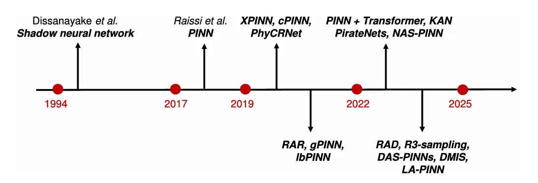
Extended PINNs (XPINNs), a generalized space-time domain decomposition approach for solving nonlinear PDEs on complex-geometry domains is proposed. Conservative PINNs (cPINNs) solves nonlinear conservation laws on discrete domains. It provides additional flexibility in choosing optimization algorithms and training parameters.

Activation functions

Nonlinear activation functions are essential in PINNs (tanh and sigmoid)

• An adaptive activation function scalable hyper-parameter for PINNs, which is dynamically adjusted during training.

  • [p] optimize the network’s topology and significantly improving convergence rates and solution accuracy Empirically, outperforms traditional fixed activation functions, especially in early training phases Gradient descent algorithms utilizes the proposed method are not attracted to suboptimal critical points or local minima

• Physics-Informed Kernel Function Neural Networks (PIKFNNs) designed to solve a variety of linear and specific nonlinear PDEs. employ a one-hidden-layer shallow neural network structure with physics-informed kernel functions as custom activation functions. incorporate PDE information, such as fundamental solutions, Green’s functions, harmonic functions, and solutions to simplified linear PDEs, enhancing the network’s ability to accurately approximate complex solutions

  • [p] significant improvements in accuracy and efficiency over traditional PINNs, particularly in handling irregular domains and complex geometries

• Physical Activation Functions (PAFs) are derived from the mathematical expressions inherent in the physical systems under study, rather than relying solely on standard activation functions like tanh or sigmoid. can be integrated into neural networks in an explicit or self-adaptive manner, with the latter allowing for automatic determination of the relative impact of PAFs for each neuron.

  • [p] significantly improve the accuracy of PINN predictions, particularly for out-of-training data, and reduce the network size by up to 75% while maintaining accuracy

• Innovative adaptive techniques to enhance the computational performance of deep neural networks in solving high-dimensional PDEs. Three key strategies adaptive loss functions, adaptive activation functions, and adaptive sampling

  • Adaptive loss function modify the traditional $L^2$ norm introducing a parameter $\alpha$ that transforms the loss function based on the training phase
  • Adaptive activation function varies the activation across layers
  • Adaptive sampling allocate more points to regions with higher local residual errors
    • [p] improve the accuracy and convergence speed of Deep Neural Networks without increasing the network complexity

Adaptive data resampling for PINN

The performance of PINNs heavily relies on the strategic selection of sampling points to effectively train the network. The location or distribution of these points is crucial for accurately approximating the solutions. In most PINNs, the collection points for training (residual points) are specified at the beginning of training and not changed during the training process. Such sampling methods can used in PINNs uniform sampling, random sampling, Latin hypercube sampling (LHS), Halton sequence, Hammersley sequence, Sobel sequence Recently, adaptive sampling strategies have been developed to dynamically adjust the distribution of sampling points based on the current state of the network’s training.

1. Residual-based adaptive refinement (RAR) adds new residual points in the locations with large PDE residuals
2. Importance sampling approach By sampling collocation points according to a distribution proportional to the loss function, this method accelerates convergence and improves training effectiveness. straightforward to implement
3. Residual-based adaptive distribution (RAD) & Residual-based adaptive refinement with distribution (RAR-D) Two nonuniform sampling techniques Dynamically adjust the distribution of residual points according to a designed probability density function (PDF) to enhance the training efficiency and accuracy of PINNs.
4. Retain-Resample-Release (R3) address the issue of propagation failures in PINNs It hypothesizes that successful training of PINNs depends on the effective propagation of solutions from initial/boundary conditions to interior points. R3 algorithm incrementally accumulates collocation points in regions of high PDE residuals, mitigating these failures with minimal computational overhead
5. Deep adaptive sampling-PINNs (DAS-PINNs) uses deep generative models to dynamically refine the training set by generating new collocation points. This method treats the residual as a PDF and uses a generative model (KRnet), to sample points consistent with this distribution-more samples are placed in regions of higher residual.
6. Dynamic mesh-based importance sampling (DMIS) address the computational inefficiency and unstable convergence issues inherent in PINN training. This method integrates importance sampling into the training process by constructing a dynamic triangular mesh that efficiently estimates sample weights.
7. Gaussian mixture distribution-based adaptive sampling (GAS) Dynamically refine the sampling of collocation points uses the current residual information to generate a Gaussian mixture distribution for sampling additional points, accelerating convergence and improving accuracy.
8. PINN adaptive collocation and experimental points selection (PINNACLE) optimize the selection of all types of training points for PINNs. focus solely on collocation or experimental points. This method jointly optimizes the selection of both, adjusting the proportion of collocation point types as training progresses.
9. Adversarial adaptive sampling (AAS) A novel method that integrates PINNs with optimal transport theory. This method employs a deep generative model to adjust the distribution of random samples in the training set, ensuring the residual induced by the neural network maintains a smooth profile. By embedding the Wasserstein distance between the residual-induced distribution and a uniform distribution into the loss function, AAS minimizes the statistical errors introduced by random samples.
10. Enhanced hybrid adaptive PINN SOTA employs a hybrid adaptive (HA) sampling method which ensures randomness in sampling points while also giving due consideration to points with large PDE residuals during the training procedure.

Loss function and Optimization for PINN

Loss function impacts convergence and the network’s ability to learn effectively.

Loss reweighting

In PINNs, the PDE loss, initial and boundary condition losses are typically added together and optimized directly. However, the scale and convergence speed of different loss terms might be different. The imbalances among these losses can lead to deteriorated performance. loss reweighting: adaptively adjust the relative importance of different components in the loss functions.

1. Examine gradient flow pathologies & Propose solutions to enhance their predictive accuracy It introduces a learning rate annealing algorithm that leverages gradient statistics to balance the composite loss functions and propose a novel neural network architecture more resilient to gradient issues. Investigate the training dynamics of PINNs using the Neural Tangent Kernel (NTK) framework. Under certain conditions, it converges to a deterministic kernel that remains constant during training in the infinite-width limit.

   • [p] This analysis with NTK reveals discrepancies in the convergence rates of different loss components.
   • [p] Improve the stability and effectiveness of PINNs (balance the training process with eigenvalues of the NTK)

2. A self-adaptive loss balanced PINNs (IbPINNs) uses a self-adaptive mechanism that dynamically adjusts the weights of the different loss terms during training. Probabilistic modeling and maximum likelihood estimation establish a Gaussian probabilistic model with output $u$. Gaussian likelihood: $p\left(u|\hat{u}(x,t;\theta )\right)=N\left(\hat{u}(x,t,;\theta ),{\epsilon }_d^2\right)$

   • PINN approximation: $\hat{u}(x,t;\theta )$
   • uncertainty parameter: ${\epsilon }_d$
   $$L(ϵ;\theta ;N)=\frac{1}{2{ϵ}_f^2}{L}_{PDE}(\theta ;N_f)+\frac{1}{2{ϵ}_b^2}{L}_{BC}(\theta ;N_b)+\frac{1}{2{ϵ}_i^2}{L}_{IC}(\theta ;N_i)+\frac{1}{2{ϵ}_d^2}{L}_{data}(\theta ;N_{data})+\log {ϵ}_f{ϵ}_b{ϵ}_i{ϵ}_d{ϵ}_d$$
   • [p] It establishes the multi-output model with four vectors to define the complex loss function.
   • [p] It have made progress in designing fast and accurate scientific machine learning technique.
   • [!] Commonly, the adaptive weight of PDE loss decreases slowly.
   • [i] Explore whether this probabilistic model is the most appropriate one, and under certain assumptions. It is possible to establish a unified framework with several other loss balancing algorithms. Different weights for each loss term can be even adjusted at each training point. SelectNet, a novel self-paced learning framework designed to improve the convergence of PINNs, prioritizes easier samples in the early stages of training and gradually incorporates more challenging ones.

3. Self-adaptive PINNs (SA-PINNs) employ fully trainable adaptation weights that apply individual attention to each training point, enabling the network to autonomously identify and focus on challenging regions of the solution. The adaptive weights create a soft attention mask, increasing as the corresponding losses increase, demonstrates how to construct a continuous map of adaptive weights using Gaussian process regression, facilitating the use of stochastic gradient descent in scenarios where conventional gradient descent is insufficient.

   • [p] improve the accuracy and robustness of PDE solutions

4. Loss-attentional PINN (LA-PINN) a novel architecture to tackle the issue that the vanilla PINN suffers from slow convergence speed and poor accuracy at hard-to-fit regions. This architecture pays attention to the control of loss error at each training point by allocating every independent loss component with a loss-attentional net (LAN) Proceeding by feeding point squared error (SE) into LAN, the attentional function could be built to accomplish the task of distributing different weights to diverse point errors. The LA-PINN architecture employs a point error-based weighting method that utilizes adversarial training between the main network and the LANs. The main network (predicting the solution): minimizes the loss through gradient descent, while the LANs adjust the weights of the SEs at these points more attention is given to hard-to-fit points by increasing the growth rates of both the weights and the update gradients for the SEs at these points

   • [p] superior predictive performance and faster convergence compared to vanilla PINNs and other SOTA methods.
   • [p] efficiency of LA-PINN in advancing the convergence of hard-to-fit points and achieving high accuracy in solving PDEs.

Novel loss functions

1. Gradient-enhanced PINNs (gPINNs) integrate gradient information into the neural network’s loss function, enhancing the model’s performance Traditional PINN: constrain the PDE residual $f$ to zero, $f(\mathbf{x})=0$, at each point $\mathbf{x}$ gPINNs: $f(\mathbf{x})=0$ + $\nabla f(\mathbf{x})=0$ The exact solution of the PDE is sufficiently smooth so that the gradient of the PDE residual exists and propose enhancing PINNs by enforcing that the derivatives of the PDE residual are also zero.

   • [p] improved accuracy, efficiency, and better generalization to regions without training points.
   • [p] require fewer training points to achieve similar or better accuracy than traditional PINNs, making them more computationally efficient. With RAR, gPINNs perform exceptionally well. A powerful tool for solving both forward and inverse PDE problems in various fields optics, fluid mechanics, system biology, and biomedicine

2. A grouping regularization strategy Conventional PINN approach & normalize the scale of different loss components This ensures that each term contributes equally to the overall loss function, thereby improving the network’s ability to capture both macroscopic and microscopic features of the solution.

   • [p] significantly outperform standard PINNs in solving multi-scale PDEs

3. Conventional use of $L^2$ loss Ubiquitous $L^2$ loss may be suboptimal & stability is achieve with sufficiently large $p$ for $L^p$ Employ a min-max optimization strategy akin to adversarial training to minimize the $L^{\infty }$

   • [p] a novel PINN training algorithm improve solution accuracy

4. loss-jump two kind of loss functions

   • Observation data loss directly constrains and measures the model output
   • Model loss includes information from governing equation and variational forms, influencing the network’s performance indirectly When transitioning from data loss to model loss, the neural network solution experiences a significant deviation from the exact solution. This phenomenon arises from the different frequency preferences of neural networks under various loss functions.

Feature embedding and augmentation

The feature (or variable) of interest is mapped into a vector space, where relationships and patterns can be more easily discerned by algorithms.

• [p] improve the performance of coordinate-based MLPs across various low-dimensional tasks in computer vision and graphics

A fundamental weakness of PINNs: spectral bias a recognized challenge in fully-connected neural networks that restricts their capacity to effectively learn high-frequency functions.

1. Spatio-temporal and multi-scale random Fourier features The coordinate embedding layers enhance the robustness and accuracy of PINN models, effectively addressing high-frequency and multi-scale challenges

2. Prior Dictionary PINN (PD-PINN) Representational power in tasks by effectively capturing features from dictionaries, thereby achieving faster convergence during training

3. sf-PINN sinusoidal mapping of inputs

   • [p] effectively increase input gradient variability
   • [p] avoid trapping in deceptive local minima

4. Dimension-augmented PINN (DaPINN) systematically manipulate the input dimensionality of the network employ spatial transformation, noise injection, color transformation, and others

   • [p] enhance the solution accuracy through replica augmentation, power series augmentation, and Fourier series augmentation
   • [p] outperform the PINN by expanding the network input dimension, which allows the neural network to extract more informative features

Challenges

1. Slow convergence, sensitivity to hyperparameters, and difficulty in scaling to high-dimensional or multi-physics problems due to the complexity of managing neural network, physics-informed loss, and the optimization methods in practice

2. A critical gradient pathologies issue that arises due to numerical stiffness, leading to imbalanced gradients during backpropagation.

   • [c] impede the network’s ability to accurately satisfy both the PDE constraints and boundary conditions, often resulting in suboptimal solutions

3. Difficulty in capturing fast-varying or high-frequency solutions Traditional optimization algorithms (Adam or L-BFGS) may struggle to converge efficiently in these scenarios, leading to poor performance or slow training. Multi-physics problem (different physical processes interact) introduce an extra layer of complexity that current optimization techniques may not handle well.

   • [?] more sophisticated loss functions, incorporating hierarchical models, or leveraging advanced optimization strategies

4. Noise or incomplete data vulnerable to errors and inconsistencies in the training data

5. Needs for high-quality datasets detailed experimental data in many scientific and engineering domains limits the potential for real-world applications

6. Highly sensitive to the choice of neural network architecture, training strategies, and the handling of boundary conditions (often require substantial tuning)

Operator learning

New paradigm that extends PINNs by focusing on learning the underlying operators governing physical systems directly

Traditional PINN

• [c] rely on solving specific PDEs or system dynamics using neural networks Operator learning
• [p] learn mappings between input and output functions (solutions to PDEs), thus enabling more generalizable models that can be applied to a wide range of physical problems without requiring explicit physics-based constraints.
• [p] More robust training algorithms capable of learning high-dimensional operator mappings efficiently (handle the complexities of multi-scale, multi-physics problems in real world applications)
• [?] Integration of data-driven and physics-based models
• [?] Explore the interpretability and explainability of models (to ensure their deployment in safety-critical engineering fields)