fourier-neural-operator

Reference

• Fourier Neural Operator for Parametric Partial Differential Equations

Tldr

learning mappings between finite-dimensional Euclidean spaces $\to$ learn the mapping from any functional parametric dependence to the solution a neural operator by parameterizing the integral kernel directly in Fourier space, allowing for an expressive and efficient architecture

Existed problems

Traditional numerical solvers are slow and sometimes inefficient. (Because systems often require fine discretization in order to compute the phenomenon being modeled.)

Conventional solvers vs. Data-driven methods

FEM (finite element methods) and FDM (finite difference methods) solve the equation by discretizing the space. coarse grids: fast but less accurate fine grids: accurate but slow Complex PDE systems usually require a very fine discretization, and therefore very challenging and time-consuming for traditional solvers. Data-driven methods can directly learn the trajectory of the family of equations from the data. Classical neural networks map between finite-dimensional spaces and can therefore only learn solutions tied to a specific discretization.

Finite-dimensional operators

These approaches parameterize the solution operator as a deep conventional neural network between finite-dimensional Euclidean spaces. Such approaches are mesh-dependent and will need modification and tunning for different resolution and discretization in order to achieve consistent error. These approaches are limited to the discretization size and geometry of the training data (and hence, it is not possible to query solutions at new points in the domain.)

Neural-FEM

directly parameterizes the solution function as a neural network This approach is designed to model one specific instance of the PDE, not the solution operator. It is mesh-independent and accurate, but for any given new instance of the functional parameter/coefficient, it requires training a new neural network. replace the linear span of a finite set of local basis functions with the space of neural networks This approach is suffers the same computational issue as classical methods (the optimization problem needs to be solved for every new instance.) (furthermore, it is limited to a setting in which the underlying PDE is known.)

Neural Operators

A new line of work proposed learning mesh-free, infinite-dimensional operators with neural networks. The neural operator remedies the mesh-dependent nature of the finite-dimensional operator methods discussed above by producing a single set of network parameters that may be used with different discretization.

• to transfer solutions between meshes
• need to be trained only once Obtaining a solution for a new instance of the parameter
• require only a forward pass of the network
• alleviate the major computational issues incurred in Neural-FEM methods
• requires no knowledge of the underlying PDE, only data Due to the cost of evaluating integral operators, neural operators have not yielded efficient numerical algorithms that can parallel the success of convolutional or recurrent neural networks in the finite-dimensional setting. However, through fast Fourier transform, FNO alleviates this issue.

Fourier Transform

The Fourier transform is frequently used in spectral methods for solving differential equations, since differentiation is equivalent to multiplication in the Fourier domain. Fourier transforms have also widely used in Deep Learning, such as

• the proof of the universal approximation theorem
• speed up convolutional neural networks
• neural network architectures involves the Fourier transform or the use of sinusoidal activation functions

Fourier Neural Operator

A novel deep learning architecture able to learn mappings between infinite-dimensional spaces of functions (the integral operator is restricted to a convolution, and instantiated through a linear transformation in the Fourier domain)

• learns the resolution-invariant solution operator where previous graph-based neural operators do not converge
• trained on a lower resolution directly evaluated on a higher resolution
• outperforms all existing deep learning methods
• increased time efficiency (2.2s $\to$ 0.005s) (no accuracy degradation)

Learning Operators

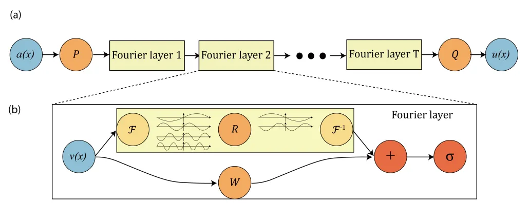a) The full architecture of neural operator input $a$

1. Lift to a higher dimension channel space by a neural network $P$
2. Apply four layers of integral operators and activation functions
3. Project back to the target dimension by a neural network $Q$ output $u$ b) Fourier layers start from input $v$ On top: apply the Fourier transform $\mathcal{F}$ (a linear transform $R$ on the lower Fourier modes and filters out the higher modes and apply the inverse Fourier transform ${\mathcal{F}}^{-1}$) On the bottom: apply a local linear transform $W$

Neural Operator

An iterative architecture $v_0\mapsto v_1\mapsto \cdots \mapsto v_T\text{where}{v}_j\text{for}j=0,1,\dots ,T-1$

Lifting

$v_0(x)=P(a(x))$ input $a$ is lifted to a higher dimensional representation by the local transformation $P$

• $P$: usually parameterized by a shallow fully-connected neural network 얇은 신경망 (shallow neural network) 인 $P$ 를 이용해 입력 데이터 $a(x)$ 의 차원을 부풀려 잠재공간 (latent space) 으로 보낸다. 신경망이 연산하기 좋게 데이터를 고차원으로 부풀린다. (신경망의 표현력 (representation capacity) 를 높임.)

Iterative operator updates

$v_{t+1}(x)=\sigma (W{v}_t(x)+\left(\mathcal{K}(a;\varphi )v_t\right)(x))$

• $W$ : linear transformation (local update)
• $\mathcal{K}(a;\varphi )$ : Kernel integral operator (global update)
• $\sigma$ : non-linear activation function Iterative updates constitute a generalization of neural networks to infinite-dimensional spaces. Even the integral operator is linear, the neural operator can learn highly non-linear operators by composing linear integral operators with non-linear activation functions (analogous to standard neural networks) $\left(\mathcal{K}(a;\varphi )v_t\right)(x):={\int }_D\kappa (x,y,a(x),a(y);\varphi )v_t(y)\mathrm{d}y$ 전체 도메인에서 상호작용하는 전역적인 (Global) 물리 법칙을 신경망의 가중치인 커널 $\mathcal{K}$ 를 통해 학습하였다. ${\kappa }_{\varphi }(x,y)={\kappa }_{\varphi }(x-y)$ Kernel integral operator = convolution operator (natural choice from the perspective of fundamental solutions) parametrizing ${\kappa }_{\varphi }$ directly in Fourier space and using the Fast Fourier Transform (FFT) to efficiently compute Kernel integral operator
• ${\kappa }_{\varphi }(x,y)$ : 위치 $y$ 에 있는 값이 위치 $x$ 에 미치는 영향
• ${\kappa }_{\varphi }(x-y)$ : 두 점의 절대적인 위치 좌표는 무시하고 두 점 사이의 거리와 방향 (상대적인 위치) 만 고려한다. 좌표만 다를 뿐, 주변 물질과 상호작용하는 물리적 규칙은 동일하다.
• $\int \kappa (x-y)v_t(y)\mathrm{d}y$ : 합성곱 $f\ast g$ 의 완벽한 정의

Convolution theorem 수학적으로 공간 도메인에서의 합성곱 연산은 주파수 도메인 (Fourier space) 에서의 단순 곱셈 연산과 같다.

1. 데이터 $v$ 를 FFT 를 통해 주파수 공간으로 넘긴다
2. 신경망이 학습할 가중치 $\mathcal{K}$ 를 아예 처음부터 주파수 공간상의 행렬 (weight) 로 만든다
3. 둘을 단순 행렬 곱셈 한다
4. 다시 IFFT (역푸리에 변환) 로 현실 공간으로 가져온다

Projection (decoding & output)

$u(x)=Q(v_T(x))$ The projection of $v_T$ by the local transformation $Q$ 여러 번의 업데이트를 거친 최종 잠재 상태 $v_T$ 를 얕은 신경망 $Q$ 를 통과시켜 다시 우리가 원하는 목표 차원으로 투영한다.

Fourier neural operator

kernel integral operator $\to$ convolution operator defined in Fourier space

• Fourier transform $(\mathcal{F}f{)}_j(k)={\int }_D{f}_j(x)e^{-2i\pi ⟨x,k⟩}\mathrm{d}x$
• Inverse Fourier transform $({\mathcal{F}}^{-1}f{)}_j(x)={\int }_D{f}_j(k)e^{2i\pi ⟨x,k⟩}\mathrm{d}k$

Prove

$\left(\mathcal{K}(a;\varphi )v_t\right)(x)={\int }_D\kappa (x,y,a(x),a(y);\varphi )v_t(y)\mathrm{d}y$ ${\kappa }_{\varphi }(x,y,a(x),a(y))={\kappa }_{\varphi }(x-y)$ $\left(\mathcal{K}(a;\varphi )v_t\right)(x)={\mathcal{F}}^{-1}(\mathcal{F}\left({\kappa }_{\varphi }\right)\cdot \mathcal{F}\left(v_t\right))(x)$

Fourier integral operator $\mathcal{K}$

$\left(\mathcal{K}(\varphi )v_t\right)(x)={\mathcal{F}}^{-1}(R_{\varphi }\cdot (\mathcal{F}{v}_t))(x)$

• $\mathcal{K}$ : Fourier integral operator
• $R_{\varphi }$ : Fourier transform of a periodic function $\kappa$ parameterized by $\varphi$ (주파수 공간의 가중치 행렬) 공간 도메인에서 커널 $\kappa$ 를 적분 (합성곱) 하는 복잡한 연산은 입력 데이터 $v_t$ 를 푸리에 변환 $\mathcal{F}$ 하고, 주파수 도메인의 가중치 행렬 $R_{\varphi }$ 를 곱한 뒤, 다시 역푸리에 변환 ${\mathcal{F}}^{-1}$ 하는 것과 완전히 똑같다. $\text{For frequency mode}k\in D,\text{we have}(\mathcal{F}{v}_t)(k)\in {\mathbb{C}}^{d_v}\text{and}{R}_{\varphi }(k)\in {\mathbb{C}}^{d_v\times d_v}$ 데이터를 Fourier transform $\mathcal{F}$ 하면 실수 세계를 떠나 복소수 세계로 간다. 파동의 크기 (진폭) 와 타이밍 (위상) 을 모두 표현해야 하기 때문이다. 특정 주파수 파동 $\kappa$ 하나를 딱 떼어놓고 보면, 데이터 $\mathcal{F}{v}_t$ 는 $d_v$ 개의 복소수 값을 가진 벡터이다. 가중치 행렬 $R_{\varphi }$ 는 $d_v\times d_v$ 크기의 복소수 행렬 ${\mathbb{C}}^{d_v\times d_v}$ 이 되어야 한다. A finite-dimensional parameterization by truncating the Fourier series at a maximal number of modes $k_{max}=|Z_{k_{max}}|$ $k_{max}$ 개의 저주파 성분만 남기고 나머지는 버린다. (Truncating) conjugate symmetry : 최종 예측 결과는 무조건 실수여야 한다. 주파수 공간에서 복소수로 계산하고, 역푸리에 변환을 ${\mathcal{F}}^{-1}$ 를 거치고 나왔을 때 허수부가 사라지고 깔끔한 실수가 나오려면 주파수 데이터가 conjugate symmetry 형태를 띠어야 한다. $Z_{k_{max}}$ : 고주파를 잘라낼 때 원형이나 마름모 형태로 잘라내는 게 수학적으로 더 이쁘장하지만, 코드로 짜기 편하게 그냥 직육면체 형태로 잘라냈다.

The discrete case and the FFT

$(R\cdot (\mathcal{F}{v}_t){)}_{k,l}={\sum }_{j=1}^{d_v}{R}_{k,l,j}(\mathcal{F}{v}_t{)}_{k,j}$Assuming the domain $D$ is discretized with $n\in \mathbb{N}$ points 현실 데이터는 연속적이지 않고 격자 (grid) 로 쪼개져 있다 Since we convolve $v_t$ with a function which only has $k_{max}$ Fourier modes, we may simply truncate the higher modes to obtain $\mathcal{F}(v_t)\in {\mathbb{C}}^{k_{max}\times d_v}$ 밑에서부터 $k_{max}$ 개의 저주파 성분만 남기고 나머지는 다 날려버린다. (==Truncation $\approx$ low band pass filter==) Multiplication by the weight tensor $R\in {\mathbb{C}}^{k_{max}\times d_v\times d_v}$

Parameterizations of $R$

$R_{\varphi }:{\mathbb{Z}}^d\times {\mathbb{R}}^d\to {\mathbb{R}}^{d_v\times d_v}$ $R$ can be defined to depend on $(\mathcal{F}a)$ to parallel $\left(\mathcal{K}(a;\varphi )v_t\right)(x)={\int }_D\kappa (x,y,a(x),a(y);\varphi )v_t(y)\mathrm{d}y$ 가중치 $R$ 을 그냥 단순한 학습 가능한 텐서로 쓴다 (=Direct parameterization) (가중치를 뱉어내는 함수로 선형 변환과 인공 신경망 두 가지를 테스트 해보았으나 결과가 좋지 않았음)

Invariance to discretization

The Fourier layers are discretization-invariant because they can learn from and evaluate functions which are discretized in an arbitrary way. Since parameters are learned directly in Fourier space, resolving the functions in physical space simply amounts to projecting on the basis $e^{2\pi ⟨x,k⟩}$ which are well-defined everywhere on ${\mathbb{R}}^d$. This allows us to achieve zero-shot super-resolution. zero-shot super-resolution : The neural operator is mesh-invariant, so it can be trained on a lower resolution and evaluated at a higher resolution, without seeing any higher resolution data. (CNN 같은 경우 해상도를 바꿀 때마다 오차가 증폭되는 치명적인 문제가 있다. 하지만 연속적인 함수 (파동) 의 매핑을 학습한 FNO 는 아무리 격자를 잘게 쪼개도 일관된 정확도를 보장한다.)

Quasi-linear complexity

General Fourier transforms complexity : $O(n^2)$ FFT complexity : $O(n\log n)$ (However, a uniform discretization is required) FFT result = DFT (Discrete Fourier Transform) result (Cooley-Tukey algorithm)

Discussion and Conclusion

Spectral analysis

The function output by $\left(\mathcal{K}(\varphi )v_t\right)(x)={\mathcal{F}}^{-1}(R_{\varphi }\cdot (\mathcal{F}{v}_t))(x)$ has at most $k_{max,j}$ Fourier modes per channel. However, this does not mean that Fourier neural operator can only approximate functions up to $k_{max,j}$ modes. Indeed, the activation functions which occur between integral operators and the final decoder network $Q$ recover the high frequency modes.

Non-periodic boundary condition

Traditional Fourier methods work only with periodic boundary conditions. However, the Fourier neural operator does not have this limitation. This is due to the linear transformation $W$ (the bias term) which keeps the track of non-periodic boundary.

Requirements on data

Data-driven methods rely on the quality and quantity of data. A future direction is to combine neural operators with numerical solvers to levitate the requirements on data.

Recurrent structure

The neural operator has an iterative structure that can naturally be formulated as a recurrent network where all layers share the same parameters without sacrificing performance.

Computer vision

Images can naturally be viewed as real-valued functions on 2-d domains and videos simply add a temporal structure. (해상도가 제각각인 카메라 영상이나 컴퓨터 비전 과제를 푸는 데 적용될 수 있음)